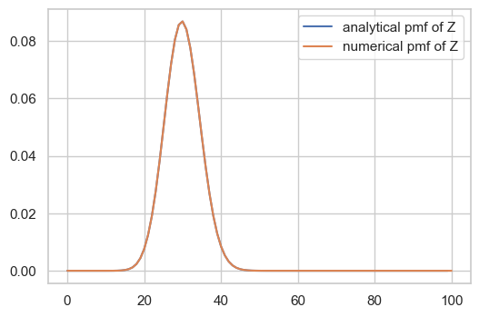
若 X 和 Y 是离散型随机变量,则 Z 的概率质量函数为 X 的概率质量函数与 Y 的概率质量函数的离散卷积:
P(Z=z)=k=−∞∑+∞P(X=k)⋅P(Y=z−k)
若 X 和 Y 是连续型随机变量,则 Z 的概率密度函数为 X 的概率密度函数与 Y 的概率密度函数的卷积:
fZ(z)=∫−∞+∞fX(x)fY(z−x)dx≡fX∗fY
卷积怎么算呢?根据定义直接算,可以,但没必要。复习一下卷积定理:
函数卷积的傅里叶变换是函数傅里叶变换的乘积。
对于离散型随机变量,我们只需要用 FFT 算法计算 X 和 Y 的概率质量函数的离散傅里叶变换,然后作乘积,再作一次逆变换,即可求得 Z 的概率质量函数。对于连续型随机变量,则可以先离散化,然后用上述方法近似求解 Z 的概率密度函数。
作为调包工程师,我们直接调用 scipy.signal.fftconvolve 实现来上述操作。
例子
我们来验证一下。
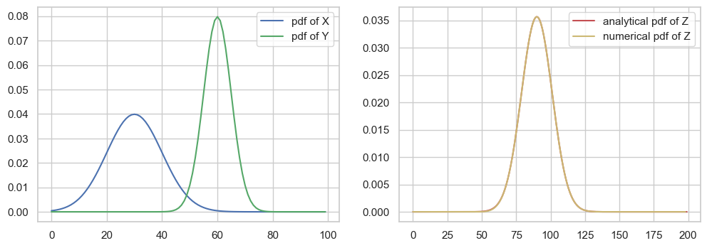
假设 X∼N(30,102),Y∼N(60,52),则 Z∼N(90,102+52)。
1
2
3
4
5
6
7
8
9
10
11
12
13
14
15
16
17
18
19
import numpy as np
import matplotlib.pyplot as plt
from scipy.stats import norm
from scipy.signal import fftconvolve

x = norm.pdf(np.arange(100), loc=30, scale=10)
y = norm.pdf(np.arange(100), loc=60, scale=5)
z = norm.pdf(np.arange(200), loc=90, scale=np.sqrt(125))
z_tilde = fftconvolve(x, y)

plt.subplot(121)
plt.plot(x, color='b', label='pdf of X')
plt.plot(y, color='g', label='pdf of Y')
plt.legend()
plt.subplot(122)
plt.plot(z, color='r', label='analytical pdf of Z')
plt.plot(z_tilde, color='y', label='numerical pdf of Z')
plt.legend()
plt.show()