指数平滑(Exponential smoothing)是除了 ARIMA 之外的另一种被广泛使用的时间序列预测方法(关于 ARIMA,请参考 时间序列模型简介)。 指数平滑即指数移动平均(exponential moving average),是以指数式递减加权的移动平均。各数值的权重随时间指数式递减,越近期的数据权重越高。常用的指数平滑方法有一次指数平滑、二次指数平滑和三次指数平滑。
1. 一次指数平滑
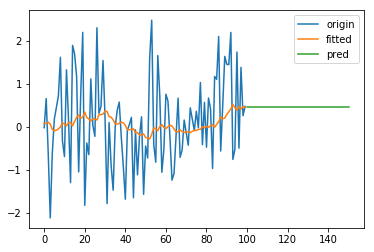
一次指数平滑又叫简单指数平滑(simple exponential smoothing, SES),适合用来预测没有明显趋势和季节性的时间序列。其预测结果是一条水平的直线。模型形如:
Forecast equation: y^t+h∣t=lt
Smoothing equantion: lt=αyt+(1−α)lt−1
其中 yt 是真实值,y^t+h(h∈Z+) 为预测值,lt 为平滑值, 0<α<1。
定义残差 ϵt=yt−y^t∣t−1,其中 t=1,⋯,T,则可以通过优化方法得到 α 和 l0。
(α∗,l0∗)=(α,l0)mint=1∑Tϵt2=(α,l0)mint=1∑T(yt−y^t∣t−1)2
使用 python 的 statsmodels 可以方便地应用该模型:
1
2
3
4
5
6
7
8
9
10
11
12
13
14
15
16
| import numpy as np
import pandas as pd
import matplotlib.pyplot as plt
from statsmodels.tsa.holtwinters import SimpleExpSmoothing
x1 = np.linspace(0, 1, 100)
y1 = pd.Series(np.multiply(x1, (x1 - 0.5)) + np.random.randn(100))
ets1 = SimpleExpSmoothing(y1)
r1 = ets1.fit()
pred1 = r1.predict(start=len(y1), end=len(y1) + len(y1)//2)
pd.DataFrame({
'origin': y1,
'fitted': r1.fittedvalues,
'pred': pred1
}).plot(legend=True)
|
效果如图:
2. 二次指数平滑
2.1 Holt’s linear trend method
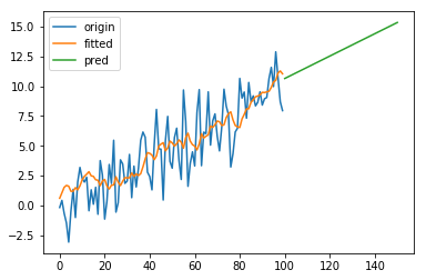
Holt 扩展了简单指数平滑,使其可以用来预测带有趋势的时间序列。直观地看,就是对平滑值的一阶差分(可以理解为斜率)也作一次平滑。模型的预测结果是一条斜率不为0的直线。模型形如:
Forecast equation: y^t+h∣t=lt+hbt
Level equation: lt=αyt+(1−α)(lt−1+bt−1)
Trend equation: bt=β(lt−lt−1)+(1−β)bt−1
其中 0<α<1, 0<β<1。
1
2
3
4
5
6
7
8
9
10
11
12
13
14
15
16
17
| import numpy as np
import pandas as pd
import matplotlib.pyplot as plt
from statsmodels.tsa.holtwinters import Holt
x2 = np.linspace(0, 99, 100)
y2 = pd.Series(0.1 * x2 + 2 * np.random.randn(100))
ets2 = Holt(y2)
r2 = ets2.fit()
pred2 = r2.predict(start=len(y2), end=len(y2) + len(y2)//2)
pd.DataFrame({
'origin': y2,
'fitted': r2.fittedvalues,
'pred': pred2
}).plot(legend=True)
|
效果如图:
2.2 Damped trend methods
Holt’s linear trend method 得到的预测结果是一条直线,即认为未来的趋势是固定的。对于短期有趋势、长期趋于稳定的序列,可以引入一个阻尼系数 0<ϕ<1,将模型改写为
Forecast equation: y^t+h∣t=lt+(ϕ+ϕ2+⋯+ϕh)bt
Level equation: lt=αyt+(1−α)(lt−1+ϕbt−1)
Trend equation: bt=β(lt−lt−1)+(1−β)ϕbt−1
3. 三次指数平滑
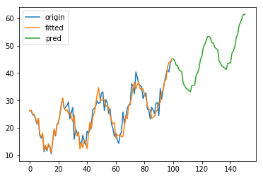
为了描述时间序列的季节性,Holt 和 Winters 进一步扩展了 Holt’s linear trend method,得到了三次指数平滑模型,也就是通常说的 Holt-Winters’ 模型。我们用 m 表示“季节”的周期。根据季节部分和非季节部分的组合方式不同,Holt-Winters’ 又可以分为加法模型和乘法模型。
3.1 Holt-Winters’ additive method
加法模型形如:
Forecast equation: y^t+h∣t=lt+hbt+st+h−m(k+1)
Level equation: lt=α(yt−st−m)+(1−α)(lt−1+bt−1)
Trend equation: bt=β(lt−lt−1)+(1−β)bt−1
Seasonal equation: st=γ(yt−lt−1−bt−1)+(1−γ)st−m
其中 0<α<1, 0<β<1,0<γ<1。k 是 mh−1 的整数部分。
1
2
3
4
5
6
7
8
9
10
11
12
13
14
15
16
17
| import numpy as np
import pandas as pd
import matplotlib.pyplot as plt
from statsmodels.tsa.holtwinters import ExponentialSmoothing
x3 = np.linspace(0, 4 * np.pi, 100)
y3 = pd.Series(20 + 0.1 * np.multiply(x3, x3) + 8 * np.cos(2 * x3) + 2 * np.random.randn(100))
ets3 = ExponentialSmoothing(y3, trend='add', seasonal='add', seasonal_periods=25)
r3 = ets3.fit()
pred3 = r3.predict(start=len(y3), end=len(y3) + len(y3)//2)
pd.DataFrame({
'origin': y3,
'fitted': r3.fittedvalues,
'pred': pred3
}).plot(legend=True)
|
效果如图:
3.2 Holt-Winters’ multiplicative method
乘法模型形如:
Forecast equation: y^t+h∣t=(lt+hbt)st+h−m(k+1)
Level equation: lt=αst−myt+(1−α)(lt−1+bt−1)
Trend equation: bt=β(lt−lt−1)+(1−β)bt−1
Seasonal equation: st=γ(lt−1+bt−1)yt+(1−γ)st−m
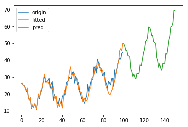
效果如图:
3.3 Holt-Winters’ damped method
Holt-Winters’ 模型的趋势部分同样可以引入阻尼系数 ϕ,这里不再赘述。
4. 参数优化和模型选择
参数优化的方法是最小化误差平方和或最大化似然函数。模型选择可以根据信息量准则,常用的有 AIC 和 BIC等。
AIC 即 Akaike information criterion, 定义为
AIC=2k−2lnL(θ)
其中 L(θ) 是似然函数, k 是参数数量。用 AIC 选择模型时要求似然函数大,同时对参数数量作了惩罚,在似然函数相近的情况下选择复杂度低的模型。
BIC 即 Bayesian information criterion,定义为
BIC=klnn−2lnL(θ)
其中 n 是样本数量。当 n>e2≈7.4 时,klnn>2k,因此当样本量较大时 BIC 对模型复杂度的惩罚比 AIC 更严厉。
5. 与 ARIMA 的关系
线性的指数平滑方法可以看作是 ARIMA 的特例。例如简单指数平滑等价于 ARIMA(0, 1, 1),Holt’s linear trend method 等价于 ARIMA(0, 2, 2),而 Damped trend methods 等价于 ARIMA(1, 1, 2) 等。
我们不妨来验证一下。
lt=αyt+(1−α)lt−1 可以改写为
y^t+1=αyt+(1−α)y^t=αyt+(1−α)(yt−ϵt)=yt−(1−α)ϵt
亦即
y^t=yt−1−(1−α)ϵt−1
两边同时加上 ϵt,得
yt=y^t+ϵt=yt−1+ϵt−(1−α)ϵt−1
而 ARIMA(p, d, q) 可以表示为
(1−i=1∑pϕiLi)(1−L)dXt=(1+i=1∑qθiLi)ϵt
其中 L 是滞后算子(Lag operator),LjXt=Xt−j。
考虑 ARIMA(0, 1, 1)
(1−L)Xt=(1+θ1L)ϵt
即
Xt−Xt−1=ϵt+θ1ϵt−1
亦即
Xt=Xt−1+ϵt+θ1ϵt−1
令 θ1=−(1−α),则两者等价。
非线性的指数平滑方法则没有对应的 ARIMA 表示。
参考文献
[1] Hyndman, Rob J., and George Athanasopoulos. Forecasting: principles and practice. OTexts, 2014.
[2] Exponential smoothing - Wikipedia
[3] Introduction to ARIMA models - Duke